Ancestral state reconstruction

Code

# code from prior sections
using CSV, DataFrames, PhyloNetworks, PhyloPlots, RCall, StatsBase, StatsModels
net = readTopology("data/polemonium_network_calibrated.phy");
for tip in net.node tip.name = replace(tip.name, r"_2$" => s""); end

We load the data at the species (morph) level and focus on log-leaflet-length, without any predictor to predict ancestral states:

traits = CSV.read("data/polemonium_traits_morph.csv", DataFrame)
subset!(traits, :morph => ByRow(in(tipLabels(net)))) # subset of rows
fit = phylolm(@formula(llength ~ 1), traits, net; tipnames=:morph,
              withinspecies_var=true, y_mean_std=true)

PhyloNetworkLinearModel

Formula: llength ~ 1

Model: Brownian motion

Parameter Estimates, using REML:
phylogenetic variance rate: 0.946928
within-species variance: 0.107488

Coefficients:
─────────────────────────────────────────────────────────────────────────
                 Coef.  Std. Error      t  Pr(>|t|)  Lower 95%  Upper 95%
─────────────────────────────────────────────────────────────────────────
(Intercept)  -0.293121    0.482432  -0.61    0.5520   -1.31583   0.729589
─────────────────────────────────────────────────────────────────────────
Log Likelihood: -334.4265947492
AIC: 674.8531894984

From the intercept coefficient we get a prediction at the root (-0.293 on the log scale) but that’s it.

predict ancestral states

This is typically called “ancestral state reconstruction” but prediction seems a more accurate term. This technique estimates the mean of nodes in the network: ancestral or extant species, conditional on the data. It’s important to look at prediction intervals, not just a “point” estimate.

asr = ancestralStateReconstruction(fit)
asr_pred = expectations(asr) # predictions at all nodes

39×2 DataFrame

14 rows omitted

Row	nodeNumber	condExpectation
	Int64	Float64
1	-5	0.257485
2	-8	-0.201828
3	7	-0.198663
4	-6	0.100981
5	-4	0.0403308
6	-10	-0.51602
7	-12	0.0315958
8	10	-0.230829
9	-15	-0.421436
10	-18	-0.130946
11	14	0.0351552
12	-20	-0.111023
13	-22	-0.326108
⋮	⋮	⋮
28	17	-0.427755
29	5	0.0306633
30	19	-1.17776
31	8	-1.05488
32	11	0.204422
33	16	0.621485
34	1	-0.863985
35	2	0.542107
36	13	0.220229
37	4	0.81878
38	6	-1.02358
39	3	0.744526

This output is somewhat cryptic though, because each row refers to a node number and it’s unclear which are tips, which are internal nodes, and which node has what number. We can also get prediction intervals (sometimes called confidence intervals) but with the same cryptic ordering of nodes:

predint(asr)

39×2 Matrix{Float64}:
 -0.522479    1.03745
 -0.79781     0.394155
 -0.790367    0.393041
 -0.691256    0.893218
 -0.657143    0.737805
 -1.31901     0.286974
 -0.828789    0.891981
 -0.939729    0.478071
 -1.12753     0.284662
 -0.89236     0.630467
 -0.671926    0.742237
 -0.762605    0.540559
 -1.00861     0.35639
  ⋮          
 -0.6454     -0.21011
 -0.067455    0.128782
 -1.56893    -0.786602
 -1.206      -0.903747
  0.0199769   0.388867
  0.579511    0.663459
 -0.944193   -0.783777
  0.489289    0.594924
  0.119035    0.321423
  0.588948    1.04861
 -1.26665    -0.780508
  0.645395    0.843657

extant species

First, we build a data frame to get this information in a more interpretable format for the tips. Below is one way to map the morph names in the order in which they appear in the data, to node numbers in the network:

tipnames_trait = traits.morph
function get_morph_nodenumber(label)
  i = findfirst(n -> n.name == label, net.node)
  net.node[i].number
end
tipnumber = [get_morph_nodenumber(label) for label in tipnames_trait]
hcat(tipnames_trait, tipnumber)

17×2 Matrix{Any}:
 "aff._viscosum_sp._nov."   12
 "apachianum"               15
 "brandegeei"               18
 "carneum"                   9
 "chartaceum"               20
 "confertum"                17
 "delicatum"                 5
 "eddyense"                 19
 "elegans"                   8
 "elusum"                   11
 "foliosissimum"            16
 "micranthum"                1
 "occidentale_occidentale"   2
 "pauciflorum"              13
 "pectinatum"                4
 "pulcherrimum_shastense"    6
 "reptans"                   3

With this mapping, we can replace the node numbers by the morph names, and add other information from the trait data such as the sample size for each morph:

tipindex_asr = indexin(tipnumber, asr_pred.nodeNumber)
res_tip = DataFrame(
      morph     = tipnames_trait, # morph names, ordered as in the trait data frame
      samplesize= traits.llength_n,
      observed  = traits.llength,
      predicted = asr_pred.condExpectation[tipindex_asr],
      low       = predint(asr)[tipindex_asr,1],
      high      = predint(asr)[tipindex_asr,2]
  )

17×6 DataFrame

Row	morph	samplesize	observed	predicted	low	high
	String31	Int64	Float64	Float64	Float64	Float64
1	aff._viscosum_sp._nov.	38	-1.371	-1.36551	-1.47801	-1.25302
2	apachianum	62	0.289364	0.287407	0.199311	0.375502
3	brandegeei	58	-0.67488	-0.673295	-0.764401	-0.582189
4	carneum	47	0.75653	0.753233	0.652009	0.854457
5	chartaceum	16	-1.61233	-1.59963	-1.77254	-1.42672
6	confertum	10	-0.430446	-0.427755	-0.6454	-0.21011
7	delicatum	50	0.0316277	0.0306633	-0.067455	0.128782
8	eddyense	3	-1.21937	-1.17776	-1.56893	-0.786602
9	elegans	21	-1.06016	-1.05488	-1.206	-0.903747
10	elusum	14	0.21314	0.204422	0.0199769	0.388867
11	foliosissimum	274	0.622095	0.621485	0.579511	0.663459
12	micranthum	75	-0.864849	-0.863985	-0.944193	-0.783777
13	occidentale_occidentale	173	0.542457	0.542107	0.489289	0.594924
14	pauciflorum	47	0.222039	0.220229	0.119035	0.321423
15	pectinatum	9	0.834157	0.81878	0.588948	1.04861
16	pulcherrimum_shastense	8	-1.04488	-1.02358	-1.26665	-0.780508
17	reptans	49	0.746643	0.744526	0.645395	0.843657

The predicted species means are close, but not exactly equal, to the observed means in each sample. This is because phylogenetic relatedness is used to share information across species. Little is shared for species with a large sample size, such as foliosissimum. But for species with a small sample size, such as eddyense, more information is borrowed from closely-related species. This is highlighted below:

filter(:morph => n -> n in ["eddyense","foliosissimum"], res_tip)

2×6 DataFrame

Row	morph	samplesize	observed	predicted	low	high
	String31	Int64	Float64	Float64	Float64	Float64
1	eddyense	3	-1.21937	-1.17776	-1.56893	-0.786602
2	foliosissimum	274	0.622095	0.621485	0.579511	0.663459

ancestral nodes

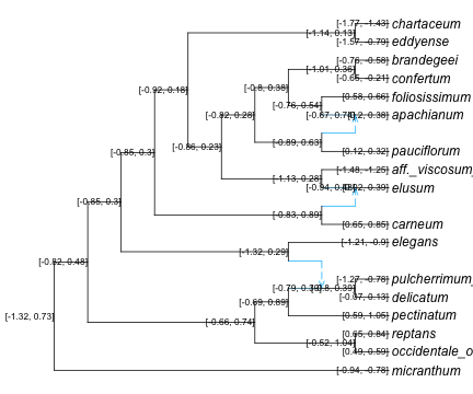
To look at ancestral states, it’s best to map the predictions and intervals onto the network. To do so, we will build a data frame containing annotations to be placed at nodes, then plot the network with this data frame as argument.

nodepred = expectationsPlot(asr)
first(nodepred, 4)

4×2 DataFrame

Row	nodeNumber	PredInt
	Int64	Abstract…
1	-5	0.26
2	-8	-0.2
3	7	-0.2
4	-6	0.1

R"par"(mar=[0,0,0,0]);
plot(net, nodelabel=nodepred, nodecex=0.8, tipoffset=0.1, xlim=[0,13]);

Figure 1: ancestral state reconstruction: species means conditional on data

nodeint = predintPlot(asr)
first(nodeint, 4)

4×2 DataFrame

Row	nodeNumber	PredInt
	Int64	Abstract…
1	-5	[-0.52, 1.04]
2	-8	[-0.8, 0.39]
3	7	[-0.79, 0.39]
4	-6	[-0.69, 0.89]

R"par"(mar=[0,0,0,0]);
plot(net, nodelabel=nodeint, nodecex=0.7, tipoffset=0.1, xlim=[-0.1,13]);

Figure 2: ancestral state reconstruction: 95% prediction interval